Mojo5 - Inverse Kinematics in Motion (#9)

I've recently implemented an inverse kinematics (IK) solution to enhance the precision and control of robotic leg movements. Our primary experiment involved programming the leg to execute a simple rectangular movement pattern, with a focus on maintaining accuracy and consistency. Here, I will share some intriguing geometrical observations and challenges we encountered.

Intended Path and Test Setup

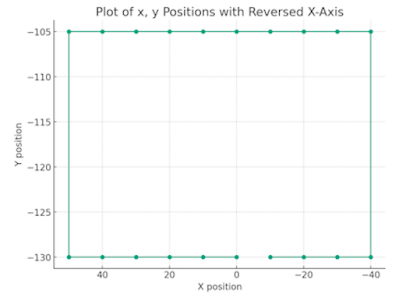
For this test, the robot leg will start in the (0,-130) position. Moving clockwise, It steps backward (in my case more positive, note the inverted x axis) to the (50, -130) position. Next up by 25mm to the top. At this time I use a different z position, but it is hard to see. the motion continues around in a rectangle ending at the start.

Planned path for simple gait test. starting at the center bottom

Video Analysis

In the bolow short video, the robot steps through the gait path. The leg is mounted above the table and horizontal to the table, not in a typical robot position. I have traced each step of the path, with a small dot at the end of the foot.

As seen in the video, the motion lacks the expected precision, influenced by several factors:

• Fixture Stability: The fixture holding the leg is unstable, contributing to erratic movements.
• Manual Marking Inaccuracy: Yellow dots indicating key positions were marked by eye, leading to imprecision.
• Servo Calibration: The calibration of the servo points was approximative. At a setting meant to be 90°, the actual angle could range between 85-95°.

Geometrical Challenges: The Skew Issue

One of the more fascinating issues we observed is the skew to the left when the leg is raised vertically. This skew is likely influenced by the constraints of the 'solution space'—the range within which the actuator operates. As a result, there is a slight warping effect in the grid area over which the leg can move.

Mojo5 Inverse Kinematics - geometric skew

Implications of the Skew

• Motor-Driven Distortions: The two servomotors, designed to drive the leg in specific rotational angles, do not guarantee a perfectly perpendicular alignment of the movement path. This introduces a mathematical distortion in the intended trajectory.
• Impact on Gait Creation: While this skew does not necessarily hinder the robot's ability to perform meaningful gaits, it highlights an essential aspect of robotic movement—geometric imperfections inherent in mechanical and software solutions.

Further Research on the Mapped or Solution Space

The space in which the robot can operates can be understood as the geometric area or volume within which the robot can effectively reach and manipulate objects. This space is defined by the following:

• Reachability: Determined by the length of the robot's arms and the range of motion of its joints. The maximum and minimum extents of each joint define the outer and inner boundaries of this space.
• Compliance: In the context of SCARA robots, the vertical compliance allows for certain movements in the vertical plane within the workspace. This selective compliance helps in absorbing forces during tasks like assembly, where vertical give is beneficial.
• Kinematic Constraints: Defined by the robot's mechanical design and the kinematic equations governing its movements. These constraints delineate the paths and patterns the robot can execute.
• Control Resolution: The precision with which the robot's controllers can position its joints also defines the resolution within the mapped space, influencing how finely the robot can maneuver within its reach.

Certainly a very interesting area of study in robotics!

Mojo5 - My Inverse Kinematics Simplified (#8)

Inverse Kinematics pictured by Dalle3, it can be much simpler!

A much simpler approach

In my previous post on Inverse Kinematics (IK), the complexity might have left some readers puzzled about whether there could be a simpler method to achieve the same results. The good news is, yes, there is a simpler way! Thanks to insights from my roboticist friend Oracid over at the French Robot Forum on Robot Maker, I've streamlined the IK calculations for our Mojo5.

Understanding the Basics

The challenge remains the same: given a target point (x, y), we need to determine the angles of the hip servo (S1) and knee servo (S2). The geometric configuration of the robot's leg has not changed; we still deal with the leg segments L1 (upper) and L2 (lower), equal in length, connected at the knee and forming two sides of a parallelogram.

Geometric Simplification

This parallelogram setup allows us to simplify our calculations considerably. The angle from the horizontal to the leg segment L1 directly provides the angle for S1, and similarly, the angle from the horizontal to the side of L2 gives us S2.

Mojo5 - simplified Inverse Kinematics

Simplified Calculation Steps

Calculate Distance D:  First, we determine the distance from the hip servo to our target (x, y) using the Pythagorean theorem:  D = sqrt(x*x + y*y).  Note D plays a very important role in the following calculations for angles alpha and beta. It is also the line that divides our parallelogram in half.

Calculate alpha:  We will use the trigonometric law of cosines. Given that we know the length of our upper leg L1 and the length of D (aka the hypotenuse), we can calculate the angle between them.  We will call this alpha:  alpha = acos(D / (2*L)).  You may notice this is the same calculation that I used previously. More importantly, this angle alpha is the same on either side of the bisection of the parallelogram by D.

Calculate beta:  We will use a much simpler approach. Also using trigonometry, we see that there is a Right Triangle formed by the Y position, X length and the hypotenuse D. it is possible to calculate this angle opposite of y and D.  beta = asin ( abs(y) / D). It must be adjusted to its reflection in the event that x < 0, this is done (in radians) by subtracting PI from beta. Now one more interesting note. The angle we just calculated is the same angle at top horizontal, this makes it more clear how this beta angle will be used in our final calculations.

Final Servo Calculations:  For S1 we can take the value of beta and subtract apha from it.  Like wise to calculate the angle for S2 and can take the value of beta and add alpha to it to find its value.

• S1 = beta - alpha
• S2 = beta + alpha

Hopefully this explaination will help in visualizing the relationships and how to calcuate the correct angles for S1 and S2.  

Here you can view a simplified set of C++ code:

void calcIK(float x, float y, float &s1, float &s2,) {

  float L = 70; //length mm

  float d = sqrt(x*x + y*y);

  float alpha = acos(d / (2*L));

  float beta = asin(abs(y)/d);  if(x<0)beta=(M_PI-beta); 

  s1 = ((beta - alpha) * (180.0 / M_PI));

  s2 = ((beta + alpha) * (180.0 / M_PI));

}